Quant Research Notes

Price as a time series

A stock does not give you one number. It gives you a sequence. For each trading day I stored a close price P(t). If Monday is t = 1 and the close is 10, then Tuesday might be 11, Wednesday 12, and so on. Almost every beginner rule I read starts from this list. Technical analysis is, at this level, just functions of past prices (Investopedia, n.d.).

I also stored a simple daily return, because later I need to grow a pretend account. The return from yesterday to today is just the percent change:

r(t) = P(t) / P(t − 1) − 1

(1) daily return

If the price goes from 10 to 11, r = 0.10, or +10%. If it goes from 11 to 10, r = −0.0909. I used this later when I compared a moving average rule to sitting in the market the whole time.

Simple moving average

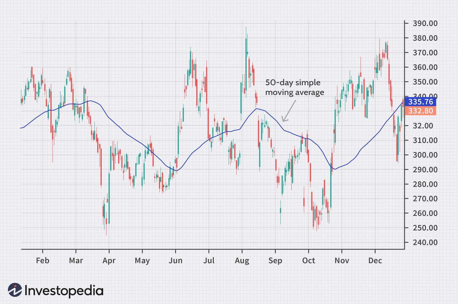
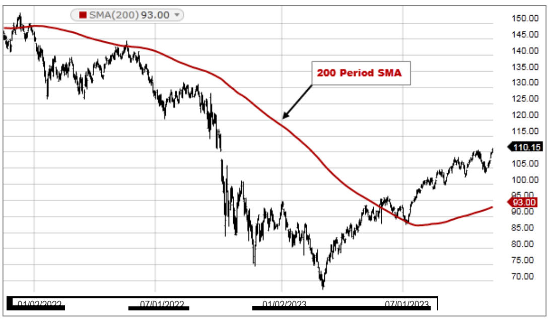
The simple moving average (SMA) is the mean of the last n closes. People use it as a smoother. A 20-day SMA is “what the last month of trading days looked like, on average.” A 50-day or 200-day SMA is slower and is often treated as a stand-in for the trend (Fidelity Learning Center, n.d.; StockCharts, n.d.).

SMAₙ(t) = (1 / n) · [P(t) + P(t − 1) + … + P(t − n + 1)]

(2) simple moving average

Worked example with n = 5. Suppose five closes are 10, 11, 12, 11, 13. The Friday SMA is (10 + 11 + 12 + 11 + 13) / 5 = 11.4. That is the entire indicator. There is no hidden step.

Day	Close	5-day SMA
Mon	10	—
Tue	11	—
Wed	12	—
Thu	11	—
Fri	13	11.4

Notice the SMA cannot exist until you have n prices. On Monday through Thursday the cell is empty. In code I skip those days so I do not pretend I had a signal I did not have. That sounds obvious, but it is a common beginner bug: filling the first days with zeros makes the program think the stock is cheap.

Figure 3. Close (navy), SMA-20 (teal), SMA-50 (grey) on my illustrative series. After the mid-sample drop, both averages keep falling for a while even if price starts to bounce. That delay is why SMA rules get in late and get out late.

Candlesticks with a 50-day simple moving average — Figure 4. A 50-day SMA drawn through candlesticks. The average is a smooth line; the candles are the noisy path. Image: Investopedia, “Moving Average (MA).”

Exponential moving average

An exponential moving average (EMA) does the same job as an SMA but gives more weight to recent days. You pick a smoothing factor α (alpha). A common choice is α = 2 / (n + 1), so a 20-day EMA uses α ≈ 0.095. Then:

EMA(t) = α · P(t) + (1 − α) · EMA(t − 1)

(3) exponential moving average

I did not use EMA as my main test because SMA is easier to show in a table. I still coded it. The practical difference is that EMA reacts a bit faster after a shock, which can help in a clean trend and can also create extra false flips in a choppy market (StockCharts, n.d.).

Crossover rules

A very old trading rule is: buy when a fast average crosses above a slow average, sell when it crosses below. People call the up-cross a “golden cross” and the down-cross a “death cross.” Brock, Lakonishok, and LeBaron (1992) tested simple versions of this on the Dow and reported that some of the rules looked better than a random walk in their sample. That paper is one of the reasons these formulas are still taught. It does not mean they still work after costs, after everyone knows them, or on every stock I pick.

A even simpler rule, which I used in Findings, is: hold the market when price is above the SMA, hold cash when it is below. Faber (2007) used a 10-month SMA on monthly data as a timing overlay. I used a 50-day SMA on daily data because I was working with a short illustrative series, not 40 years of monthly index levels.

Price with a 200-day simple moving average — Figure 5. A long 200-day SMA. Price spent a long stretch below the line, then recovered through it. Image: Fidelity Learning Center, “Simple Moving Average.”

Relative Strength Index

RSI was described by J. Welles Wilder (1978). It tries to measure how one-sided recent moves have been. First you split each daily change into a gain or a loss. Then you average those over n days (Wilder used n = 14). Relative strength is the ratio of average gain to average loss. RSI rescales that ratio onto 0 to 100.

RS = average gain / average loss

(4) relative strength

RSI = 100 − 100 / (1 + RS)

(5) RSI

If every day is an up day, average loss is near zero and RSI is near 100. If every day is a down day, RSI is near 0. Wilder’s original notes treated RSI above 70 as “overbought” and below 30 as “oversold.” Quantpedia and later timing papers also use RSI in a different way: as a trend filter, for example staying long when a slow RSI is above 50 (Quantpedia, 2023). Those are two different jobs — mean reversion versus trend — using the same number.

Figure 6. 14-day RSI on the same series. Dashed lines at 70 and 30. The middle of the sample spends a lot of time under 30, which matches the price drop in Figure 3. I did not trade every touch of 30. I only plotted it so I could see the formula move.

A thing I had to be careful about: Wilder’s smoothing is recursive, like an EMA of gains and losses. If I used a plain SMA of the last 14 changes, I get a close cousin called Cutler’s RSI. For a student project the difference is small. I used the recursive version so the code matches the usual write-up.

Volatility, in one line

Volatility here just means “how jumpy are the returns.” The version I used is the sample standard deviation of daily r(t), sometimes multiplied by the square root of 252 if I want a yearly number (because there are about 252 trading days in a year):

σ_ann ≈ stdev(r) · √252

(6) annualized volatility

I am not using this as a trading signal. I am using it as a warning. A rule that looks good because it sat out one crash still has to be judged by how much the account bounced around on the days it was in. Findings reports a rough drawdown next to return for that reason.